

Let's see here as to how we can lock rows and columns in MS Excel 2007. Locking rows and columns in an excel language is referred as “Freeze Panes”. You can either lock the entire row or lock the entire column or lock both row and column together.
Below you can see the database which we will be using to demonstrate how we lock rows and columns.
 Now suppose you need to enter more data, below the last entry which in this case is 25th. So, as soon as you scroll down, the heading of the database gets hidden as it also gets scrolled up.
This is what happens:
Now suppose you need to enter more data, below the last entry which in this case is 25th. So, as soon as you scroll down, the heading of the database gets hidden as it also gets scrolled up.
This is what happens:
 In order to prevent this from happening, Microsoft Excel has a wonderful feature called “Freeze Panes”. In order to freeze panes or what generally people refer to as locking rows and columns, this is what you need to do:
From the place where you need to lock the row take your cursor just below that row in the first column. So here we need to lock the first row therefore lets take our cursor to the second cell in the first column just below the row which needs to be locked. Here the cell is A2.
In order to prevent this from happening, Microsoft Excel has a wonderful feature called “Freeze Panes”. In order to freeze panes or what generally people refer to as locking rows and columns, this is what you need to do:
From the place where you need to lock the row take your cursor just below that row in the first column. So here we need to lock the first row therefore lets take our cursor to the second cell in the first column just below the row which needs to be locked. Here the cell is A2.
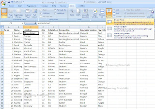
 Once you have placed you cursor at the right place. Follow the steps mentioned below:
• Point “View” from the menu.
• Click on “Freeze Panes” under “Window” option
• Select “Freeze Panes”
Once you have placed you cursor at the right place. Follow the steps mentioned below:
• Point “View” from the menu.
• Click on “Freeze Panes” under “Window” option
• Select “Freeze Panes”
 And you are done! You have successfully locked the top row. Now no matter how much you scroll down you wont loose out on the header.
 In order to lock columns you need to follow the same steps which we did to lock rows.
We have an option to lock the first column. In order to lock the first column, which here is, “Sr No” do the following:
• Irrespective of wherever your cursor is placed, Point to View .
• Click on “Freeze Panes” under “Window” option.
• Select “Freeze First Column”
In order to lock columns you need to follow the same steps which we did to lock rows.
We have an option to lock the first column. In order to lock the first column, which here is, “Sr No” do the following:
• Irrespective of wherever your cursor is placed, Point to View .
• Click on “Freeze Panes” under “Window” option.
• Select “Freeze First Column”
 And you are done with, locking the first column of your sheet.
 In order to lock a column just take the cursor to the first cell of the column next to the column which has to be locked. Here we are trying to lock the “Age” column, so let us take the cursor to cell E1.
After pointing cell E1 point to “View” then click on “Freeze Panes” option and click on “Freeze Panes”
In order to lock a column just take the cursor to the first cell of the column next to the column which has to be locked. Here we are trying to lock the “Age” column, so let us take the cursor to cell E1.
After pointing cell E1 point to “View” then click on “Freeze Panes” option and click on “Freeze Panes”
 And here we are done with freezing the columns. How much ever we may scroll right, we will be able to see the age column.
Just a point to be kept in mind: Whenever we freeze either a row or a column all the rows above it and all the columns to the left of the freezed ones also remain freezed.
Next we will demonstrate how do we freeze both row and column together. This can be done the following way: Once you have decided which row and which column you need to lock take your cursor to the cell just below their intersection.
Let’s say for example we need the "Sr No" and "Name" column always visible and the top row always visible. In order to do that go to the cell below their intersection. Here it is cell C2 and point to “View” menu and click on “Freeze Panes” Option and click “Freeze Panes”.
And here we are done with freezing the columns. How much ever we may scroll right, we will be able to see the age column.
Just a point to be kept in mind: Whenever we freeze either a row or a column all the rows above it and all the columns to the left of the freezed ones also remain freezed.
Next we will demonstrate how do we freeze both row and column together. This can be done the following way: Once you have decided which row and which column you need to lock take your cursor to the cell just below their intersection.
Let’s say for example we need the "Sr No" and "Name" column always visible and the top row always visible. In order to do that go to the cell below their intersection. Here it is cell C2 and point to “View” menu and click on “Freeze Panes” Option and click “Freeze Panes”.
 Now how much ever you may scroll right or how much ever you may scroll down, you will never lose out on the header or on the Name column.
 Tip: The shortcut to lock (Freeze) and unlock (Unfreeze) either rows or column or both is Alt+W+F+F
 Now suppose you need to enter more data, below the last entry which in this case is 25th. So, as soon as you scroll down, the heading of the database gets hidden as it also gets scrolled up.
This is what happens:
Now suppose you need to enter more data, below the last entry which in this case is 25th. So, as soon as you scroll down, the heading of the database gets hidden as it also gets scrolled up.
This is what happens:
 In order to prevent this from happening, Microsoft Excel has a wonderful feature called “Freeze Panes”. In order to freeze panes or what generally people refer to as locking rows and columns, this is what you need to do:
From the place where you need to lock the row take your cursor just below that row in the first column. So here we need to lock the first row therefore lets take our cursor to the second cell in the first column just below the row which needs to be locked. Here the cell is A2.
In order to prevent this from happening, Microsoft Excel has a wonderful feature called “Freeze Panes”. In order to freeze panes or what generally people refer to as locking rows and columns, this is what you need to do:
From the place where you need to lock the row take your cursor just below that row in the first column. So here we need to lock the first row therefore lets take our cursor to the second cell in the first column just below the row which needs to be locked. Here the cell is A2.
 Once you have placed you cursor at the right place. Follow the steps mentioned below:
• Point “View” from the menu.
• Click on “Freeze Panes” under “Window” option
• Select “Freeze Panes”
Once you have placed you cursor at the right place. Follow the steps mentioned below:
• Point “View” from the menu.
• Click on “Freeze Panes” under “Window” option
• Select “Freeze Panes”
 And you are done! You have successfully locked the top row. Now no matter how much you scroll down you wont loose out on the header.
 In order to lock columns you need to follow the same steps which we did to lock rows.
We have an option to lock the first column. In order to lock the first column, which here is, “Sr No” do the following:
• Irrespective of wherever your cursor is placed, Point to View .
• Click on “Freeze Panes” under “Window” option.
• Select “Freeze First Column”
In order to lock columns you need to follow the same steps which we did to lock rows.
We have an option to lock the first column. In order to lock the first column, which here is, “Sr No” do the following:
• Irrespective of wherever your cursor is placed, Point to View .
• Click on “Freeze Panes” under “Window” option.
• Select “Freeze First Column”
 And you are done with, locking the first column of your sheet.
 In order to lock a column just take the cursor to the first cell of the column next to the column which has to be locked. Here we are trying to lock the “Age” column, so let us take the cursor to cell E1.
After pointing cell E1 point to “View” then click on “Freeze Panes” option and click on “Freeze Panes”
In order to lock a column just take the cursor to the first cell of the column next to the column which has to be locked. Here we are trying to lock the “Age” column, so let us take the cursor to cell E1.
After pointing cell E1 point to “View” then click on “Freeze Panes” option and click on “Freeze Panes”
 And here we are done with freezing the columns. How much ever we may scroll right, we will be able to see the age column.
Just a point to be kept in mind: Whenever we freeze either a row or a column all the rows above it and all the columns to the left of the freezed ones also remain freezed.
Next we will demonstrate how do we freeze both row and column together. This can be done the following way: Once you have decided which row and which column you need to lock take your cursor to the cell just below their intersection.
Let’s say for example we need the "Sr No" and "Name" column always visible and the top row always visible. In order to do that go to the cell below their intersection. Here it is cell C2 and point to “View” menu and click on “Freeze Panes” Option and click “Freeze Panes”.
And here we are done with freezing the columns. How much ever we may scroll right, we will be able to see the age column.
Just a point to be kept in mind: Whenever we freeze either a row or a column all the rows above it and all the columns to the left of the freezed ones also remain freezed.
Next we will demonstrate how do we freeze both row and column together. This can be done the following way: Once you have decided which row and which column you need to lock take your cursor to the cell just below their intersection.
Let’s say for example we need the "Sr No" and "Name" column always visible and the top row always visible. In order to do that go to the cell below their intersection. Here it is cell C2 and point to “View” menu and click on “Freeze Panes” Option and click “Freeze Panes”.
 Now how much ever you may scroll right or how much ever you may scroll down, you will never lose out on the header or on the Name column.
 Tip: The shortcut to lock (Freeze) and unlock (Unfreeze) either rows or column or both is Alt+W+F+F